It has been quite some time since I last posted a blog, this is mainly due to my TIMMINS One Name Study taking up more time than expected. I am still learning about surname studies so have been reading up on the subject. I have just finished the Surname Detective by Colin D. Rogers, this book has proved to be a very useful introduction as well interesting, I can recommend it if you are in any way interested in surnames. Next on my reading list is a book referred to many times by Rogers – The Origin of English Surnames by P.H Reaney.
So what else have I been doing over the past few weeks. One thing that cropped up was a requirement to investigate a surname in my wife’s family, this was subsequent to the discovery of a photograph that had a list of names on it. The family name was WARNER, they had resided in India in the 19th and early 20th century’s.
FamilySearch has pretty good coverage of India, so some family reconstruction could be carried out to determine the family groups. Searching on India Marriages for WARNER produced some 253 matches, that is 13 pages of links at 20 links per page. Each marriage record has 24 items so copy and pasting all this into an Excel spreadsheet could take a long time; but……
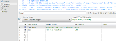
by using my favourite data capture program Outwit Hub I devised a really simple scraper and saved myself hours.
The methodology of using this scraper is the same as detailed in my previous post Extracting Marriage Data Made Easy
Once I had Caught the data in the Catch area it was exported into Excel, I then made a copy of the worksheet (this is so that I can work on the data but retain the original data – just in case!). There are a number of colums of data that I don’t need so all those are deleted, that just leaves the field name in column A and the data in column B.
I was now faced with a vertically tablulated column of data stretching over 6,072 rows (253 x 24). What I really need is 24 columns of data over 253 rows. I have used Excel for many years but my expertise in Excel functions would not enable me to sort this one out! I did know however that a macro in VBA would be my best bet, so I searched the usual forums and found a solution.
To make this macro work I needed an end of record identifier for each of the 253 records. The last field on each of the record sets was “Reference Number”, this field had no useful data in it – so I filtered column A on this field and filled all 253 instances with an “@” symbol, this this is the end of record delimiter for the macro. Column A is now no use so it is deleted. All the useful data should now be in Column A (unfiltered). Run the macro and you now have the data in a usable format. Insert a row at the top and name the columns a required. Rather than have a load of screen shots of Excel showing the process you can download the Excel Spreadsheet from my Google Documents HERE (under File – Download).
There are 4 tabs in the workbook with the instructions on how to use it in the first tab. If you want to see the code behind the macro then go to Tools – Macro – Visual Basic Editor – if it is not already visible then double click Module 1.
Well there it is, with this macro you should be able to tackle any vertically tabulated column of data and manipulate it into a useable database.
Before I sign off thanks go to Jerry Beaucaire on the Excel Forum for the neat peice of code. Jerry also has his own Excel Assistant web site where you can leave a donation if you found this code useful.


